Measures of Central Tendency
Measures of central tendency are numbers that tend to cluster around the “middle” of a set of values. Three such middle numbers are the mean, the median, and the mode.
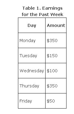
For example, suppose your earnings for the past week were the values shown in Table 1.

Mean
You could express your daily earnings from Table 1 in a number of ways. One way is to use the average, or mean, of the data set. The arithmetic mean is the sum of the measures in the set divided by the number of measures in the set. Totaling all the measures and dividing by the number of measures, you get $1,000 ÷ 5 = $200.
Median
Another measure of central tendency is the median, which is defined as the middle value when the numbers are arranged in increasing or decreasing order. When you order the daily earnings shown in Table 1, you get $50, $100, $150, $350, and $350. The middle value is $150; therefore, $150 is the median.
If there is an even number of items in a set, the median is the average of the two middle values. For example, if we had four values—4, 10, 12, and 26—the median would be the average of the two middle values, 10 and 12; in this case, 11 is the median. The median may sometimes be a better indicator of central tendency than the mean, especially when there are outliers, or extreme values.
Example 1
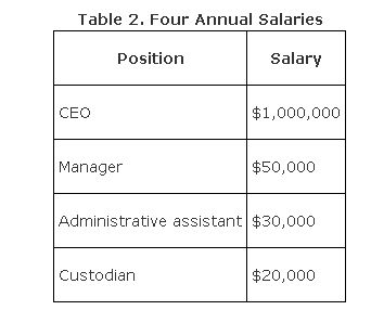
Given the four annual salaries of a corporation shown in Table 2, determine the mean and the median.
The mean of these four salaries is $275,000. The median is the average of the middle two salaries, or $40,000. In this instance, the median appears to be a better indicator of central tendency because the CEO's salary is an extreme outlier, causing the mean to lie far from the other three salaries.

Mode
Another indicator of central tendency is the mode, or the value that occurs most often in a set of numbers. In the set of weekly earnings in Table 1, the mode would be $350 because it appears twice and the other values appear only once.
Notation and formulae
The mean of a sample is typically denoted as  (read as x bar). The mean of a population is typically denoted as μ (pronounced mew). The sum (or total) of measures is typically denoted with a Σ. The formula for a sample mean is

where n is the number of values.
Mean for grouped data
Occasionally, you may have data that consist not of actual values but rather of grouped measures. For example, you may know that, in a certain working population, 32 percent earn between $25,000 and $29,999; 40 percent earn between $30,000 and $34,999; 27 percent earn between $35,000 and $39,999; and the remaining 1 percent earn between $80,000 and $85,000. This type of information is similar to that presented in a frequency table. Although you do not have precise individual measures, you still can compute measures for grouped data, data presented in a frequency table.
The formula for a sample mean for grouped data is

where x is the midpoint of the interval, f is the frequency for the interval, fx is the product of the midpoint times the frequency, and n is the number of values.
For example, if 8 is the midpoint of a class interval and there are ten measurements in the interval, fx = 10(8) = 80, the sum of the ten measurements in the interval.
Σ fx denotes the sum of all the products in all class intervals. Dividing that sum by the number of measurements yields the sample mean for grouped data.
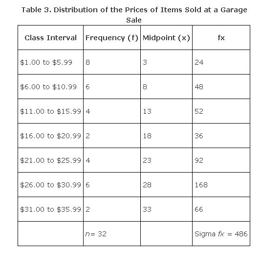
For example, consider the information shown in Table 3.

Substituting into the formula:

Therefore, the average price of items sold was about $15.19. The value may not be the exact mean for the data, because the actual values are not always known for grouped data.
Median for grouped data
As with the mean, the median for grouped data may not necessarily be computed precisely because the actual values of the measurements may not be known. In that case, you can find the particular interval that contains the median and then approximate the median.
Using Table 3, you can see that there is a total of 32 measures. The median is between the 16th and 17th measure; therefore, the median falls within the $11.00 to $15.99 interval. The formula for the best approximation of the median for grouped data is

where L is the lower class limit of the interval that contains the median, n is the total number of measurements, w is the class width, f medis the frequency of the class containing the median, and Σ f b is the sum of the frequencies for all classes before the median class.
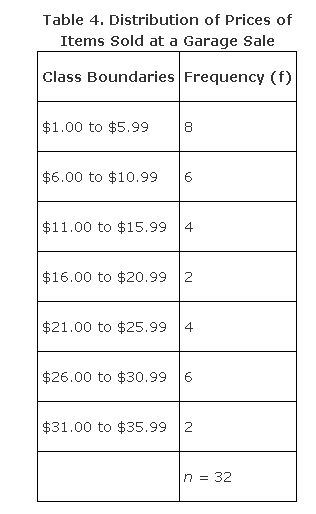
Consider the information in Table 4.

As we already know, the median is located in class interval $11.00 to $15.99. So L = 11, n = 32, w = 4.99, f med = 4, and Σ f b = 14.
Substituting into the formula:

Symmetric distribution
In a distribution displaying perfect symmetry, the mean, the median, and the mode are all at the same point, as shown in Figure 1.
Figure 1.For a symmetric distribution, mean, median, and mode are equal.

Skewed curves
As you have seen, an outlier can significantly alter the mean of a series of numbers, whereas the median will remain at the center of the series. In such a case, the resulting curve drawn from the values will appear to be skewed, tailing off rapidly to the left or right. In the case of negatively skewed or positively skewed curves, the median remains in the center of these three measures.
Figure 2 shows a negatively skewed curve.
Figure 2.A negatively skewed distribution, mean < median < mode.

Figure 3 shows a positively skewed curve.
Figure 3.A positively skewed distribution, mode < median < mean.

|
|
|
|
|
|
|
|
|
|
|
|
|
|
|
|
|
|
|
|
|