You have been using probability to decide whether a statistical test provides evidence for or against your predictions. If the likelihood of obtaining a given test statistic from the population is very small, you reject the null hypothesis and say that you have supported your hunch that the sample you are testing is different from the population.
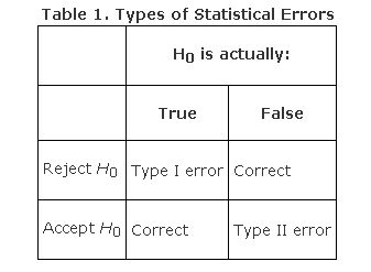
But you could be wrong. Even if you choose a probability level of 5 percent, that means there is a 5 percent chance, or 1 in 20, that you rejected the null hypothesis when it was, in fact, correct. You can err in the opposite way, too; you might fail to reject the null hypothesis when it is, in fact, incorrect. These two errors are called Type I and Type II, respectively. Table 1 presents the four possible outcomes of any hypothesis test based on (1) whether the null hypothesis was accepted or rejected and (2) whether the null hypothesis was true in reality.

A Type I error is often represented by the Greek letter alpha (α) and a Type II error by the Greek letter beta (β ). In choosing a level of probability for a test, you are actually deciding how much you want to risk committing a Type I error—rejecting the null hypothesis when it is, in fact, true. For this reason, the area in the region of rejection is sometimes called the alpha level because it represents the likelihood of committing a Type I error.
In order to graphically depict a Type II, or β, error, it is necessary to imagine next to the distribution for the null hypothesis a second distribution for the true alternative (see Figure 1). If the alternative hypothesis is actually true, but you fail to reject the null hypothesis for all values of the test statistic falling to the left of the critical value, then the area of the curve of the alternative (true) hypothesis lying to the left of the critical value represents the percentage of times that you will have made a Type II error.
Figure 1.Graphical depiction of the relation between Type I and Type II errors, and the power of the test.

Type I and Type II errors are inversely related: As one increases, the other decreases. The Type I, or α (alpha), error rate is usually set in advance by the researcher. The Type II error rate for a given test is harder to know because it requires estimating the distribution of the alternative hypothesis, which is usually unknown.
A related concept is power—the probability that a test will reject the null hypothesis when it is, in fact, false. You can see from Figure 1 that power is simply 1 minus the Type II error rate (β). High power is desirable. Like β, power can be difficult to estimate accurately, but increasing the sample size always increases power.
|
|