Aggregate Supply (AS) Curve
The aggregate supply curve depicts the quantity of real GDP that is supplied by the economy at different price levels. The reasoning used to construct the aggregate supply curve differs from the reasoning used to construct the supply curves for individual goods and services. The supply curve for an individual good is drawn under the assumption that input prices remain constant. As the price of good X rises, sellers' per unit costs of providing good X do not change, and so sellers are willing to supply more of good X‐hence, the upward slope of the supply curve for good X. The aggregate supply curve, however, is defined in terms of the price level. Increases in the price level will increase the price that producers can get for their products and thus induce more output. But an increase in the price will also have a second effect; it will eventually lead to increases in input prices as well, which, ceteris paribus, will cause producers to cut back. So, there is some uncertainty as to whether the economy will supply more real GDP as the price level rises. In order to address this issue, it has become customary to distinguish between two types of aggregate supply curves, the short‐run aggregate supply curve and the long‐run aggregate supply curve.
Short‐run aggregate supply curve. The short‐run aggregate supply (SAS) curve is considered a valid description of the supply schedule of the economy only in the short‐run. The short‐run is the period that begins immediately after an increase in the price level and that ends when input prices have increased in the same proportion to the increase in the price level.
Input prices are the prices paid to the providers of input goods and services. These input prices include the wages paid to workers, the interest paid to the providers of capital, the rent paid to landowners, and the prices paid to suppliers of intermediate goods. When the price level of final goods rises, the cost of living increases for those who provide input goods and services. Once these input providers realize that the cost of living has increased, they will increase the prices that they charge for their input goods and services in proportion to the increase in the price level for final goods.
The presumption underlying the SAS curve is that input providers do not or cannot take account of the increase in the general price level right away so that it takes some time–referred to as the short‐run–for input prices to fully reflect changes in the price level for final goods. For example, workers often negotiate multi‐year contracts with their employers. These contracts usually include a certain allowance for an increase in the price level, called a cost of living adjustment (COLA). The COLA, however, is based on expectations of the future price level that may turn out to be wrong. Suppose, for example, that workers underestimate the increase in the price level that occurs during the multi‐year contract. Depending on the terms of the contract, the workers may not have the opportunity to correct their mistaken estimates of inflation until the contract expires. In this case, their wage increases will lag behind the increases in the price level for some time.
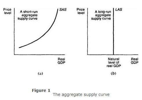
During the short‐run, sellers of final goods are receiving higher prices for their products, without a proportional increase in the cost of their inputs. The higher the price level, the more these sellers will be willing to supply. The SAS curve—depicted in Figure (a)—is therefore upward sloping, reflecting the positive relationship that exists between the price level and the quantity of goods supplied in the short‐run.

Long‐run aggregate supply curve. The long‐run aggregate supply (LAS) curve describes the economy's supply schedule in the long‐run. The long‐run is defined as the period when input prices have completely adjusted to changes in the price level of final goods. In the long‐run, the increase in prices that sellers receive for their final goods is completely offset by the proportional increase in the prices that sellers pay for inputs. The result is that the quantity of real GDP supplied by all sellers in the economy is independent of changes in the price level. The LAS curve—depicted in Figure (b)—is a vertical line, reflecting the fact that long‐run aggregate supply is not affected by changes in the price level. Note that the LAS curve is vertical at the point labeled as the natural level of real GDP. The natural level of real GDP is defined as the level of real GDP that arises when the economy is fully employing all of its available input resources.
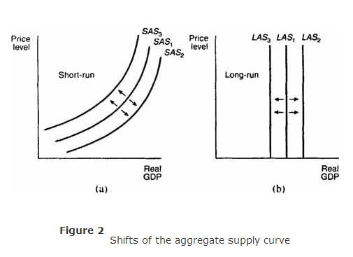
Changes in aggregate supply. Changes in aggregate supply are represented by shifts of the aggregate supply curve. An illustration of the ways in which the SAS and LAS curves can shift is provided in Figures (a) and (b). A shift to the right of the SAS curve from SAS 1 to SAS 2 of the LAS curve from LAS 1 to LAS 2 means that at the same price levels the quantity supplied of real GDP has increased. A shift to the left of the SAS curve from SAS 1 to SAS 3 or of the LAS curve from LAS 1 to LAS 3 means that at the same price levels the quantity supplied of real GDP has decreased .


Like changes in aggregate demand, changes in aggregate supply are not caused by changes in the price level. Instead, they are primarily caused by changes in two other factors. The first of these is a change in input prices. For example, the price of oil, an input good, increased dramatically in the 1970s due to efforts by oil‐exporting countries to restrict the quantity of oil sold. Many final goods and services use oil or oil products as inputs. Suppliers of these final goods and services faced rising costs and had to reduce their supply at all price levels. The decrease in aggregate supply, caused by the increase in input prices, is represented by a shift to the left of the SAS curve because the SAS curve is drawn under the assumption that input prices remain constant. An increase in aggregate supply due to a decrease in input prices is represented by a shift to the right of the SAS curve.
A second factor that causes the aggregate supply curve to shift is economic growth. Positive economic growth results from an increase in productive resources, such as labor and capital. With more resources, it is possible to produce more final goods and services, and hence, the natural level of real GDP increases. Positive economic growth is therefore represented by a shift to the right of the LAS curve. Similarly, negative economic growth decreases the natural level of real GDP, causing the LAS curve to shift to the left.