Combining AD and AS Supply Curves
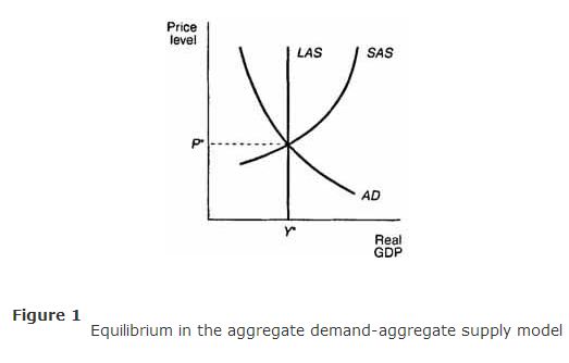
When the aggregate demand and SAS (short-run aggregate supply) curves are combined, as in Figure , the intersection of the two curves determines both the equilibrium price level, denoted by P *, and the equilibrium level of real GDP, denoted by Y * .


If it is further assumed that the economy is fully employing all of its resources, the equilibrium level of real GDP, Y *, will correspond to the natural level of real GDP, and the LAS curve may be drawn as a vertical line at Y *, as in Figure .
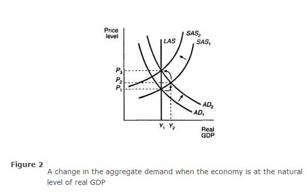
Consider what happens to this situation when the aggregate demand curve shifts to the right from AD 1 toAD 2, as in Figure .

The immediate, short‐run effect is that the equilibrium price level increases from P 1, to P 2, and real GDP increases above its natural level, from Y 1, to Y 2 . The increase in real GDP is due to the fact that input prices have not yet risen in response to the increase in the price level for final goods; the economy is still operating along the old SAS curve, SAS 1 . Eventually, however, input providers will demand higher prices to reflect the increase in the general price level. Production costs will therefore increase, and the supply of real GDP will be reduced. This is represented by the shift to the left of the SAS curve from SAS 1 to SAS 2. The end result is a higher price level, P 3, at the same, natural level of real GDP, Y 1.
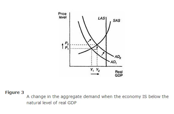
The graphical analysis presented in Figure applies only to the case where there is zero economic growth, and the economy is already at the natural level of real GDP when aggregate demand increases. In the case where the economy is not fully employing all of its input resources and has therefore not yet attained its natural level of real GDP, an increase in aggregated demand—depicted in Figure as a shift from AD 1 to AD 2—causes both an increase in the equilibrium price level from P 1 to P 2, and an increase in the equilibrium level of real GDP from Y 1 to Y 2 .

In this case, the increase in the equilibrium price level does not necessarily lead to an increase in input prices because the economy is not fully employing all of its input resources. When unemployed inputs are available, input prices do not tend to rise. The result, in this case, is that the SAS curve does not shift left and cancel out the increase in real GDP brought about by the increase in aggregate demand.